

Simple Price Prediction Model
Prediction of Flight Price:
Predicting the price of a flight fare on the basis of several parameters such as Flight Org,Date,Stops etc. Which depicts that it’s a regression problem. Starting with the required library imports.
import numpy as np
import pandas as pd
import matplotlib.pyplot as plt
import seaborn as sns
import matplotlib.style as style
import missingno as msno
sns.set()
Load the dataset and perform the basic data validations.As we have date and time columns so we should parse it at load time.
train_data = pd.read_csv("data_train.csv",parse_dates=['Date_of_Journey','Dep_Time','Arrival_Time'])
pd.set_option('display.max_columns', None)
train_data.head()
| Airline | Date_of_Journey | Source | Destination | Route | Dep_Time | Arrival_Time | Duration | Total_Stops | Additional_Info | Price | |
|---|---|---|---|---|---|---|---|---|---|---|---|
| 0 | IndiGo | 2019-03-24 | Banglore | New Delhi | BLR ? DEL | 2020-07-13 22:20:00 | 2020-03-22 01:10:00 | 2h 50m | non-stop | No info | 3897 |
| 1 | Air India | 2019-01-05 | Kolkata | Banglore | CCU ? IXR ? BBI ? BLR | 2020-07-13 05:50:00 | 2020-07-13 13:15:00 | 7h 25m | 2 stops | No info | 7662 |
| 2 | Jet Airways | 2019-09-06 | Delhi | Cochin | DEL ? LKO ? BOM ? COK | 2020-07-13 09:25:00 | 2020-06-10 04:25:00 | 19h | 2 stops | No info | 13882 |
| 3 | IndiGo | 2019-12-05 | Kolkata | Banglore | CCU ? NAG ? BLR | 2020-07-13 18:05:00 | 2020-07-13 23:30:00 | 5h 25m | 1 stop | No info | 6218 |
| 4 | IndiGo | 2019-01-03 | Banglore | New Delhi | BLR ? NAG ? DEL | 2020-07-13 16:50:00 | 2020-07-13 21:35:00 | 4h 45m | 1 stop | No info | 13302 |
Validating the possibilities of null values and from the plot we confirm that there are very marginal missing values.
msno.matrix(train_data)
<matplotlib.axes._subplots.AxesSubplot at 0x1a307d06108>

train_data.isnull().sum()
Airline            0
Date_of_Journey    0
Source             0
Destination        0
Route              1
Dep_Time           0
Arrival_Time       0
Duration           0
Total_Stops        1
Additional_Info    0
Price              0
dtype: int64
inplace is set to True means it will make the changes to the master data frame.
train_data.dropna(inplace=True)
Convert the Date_of_Journey to Day and Month
train_data["Journey_day"] =train_data["Date_of_Journey"].dt.day
train_data["Journey_month"] =train_data["Date_of_Journey"].dt.month
Now we got the day and month then we can simply drop the Date of Journey and perform the similar operation with Time.
train_data.drop(["Date_of_Journey"],axis=1,inplace=True)
# Extracting Hours
train_data["Dep_hour"] = train_data["Dep_Time"].dt.hour

# Extracting Minutes
train_data["Dep_min"] = train_data["Dep_Time"].dt.minute
train_data.drop(["Dep_Time"],axis=1,inplace=True)
Similarly we can extract values from Arrival_Time
# Extracting Hours
train_data["Arrival_hour"] = train_data["Arrival_Time"].dt.hour

# Extracting Minutes
train_data["Arrival_min"] = train_data["Arrival_Time"].dt.minute

train_data.drop(["Arrival_Time"], axis = 1, inplace = True)
hrs=[]
mins=[]
for val in train_data['Duration']:
    if len(val.split())>1:
        hr=int(val.split()[0].strip().replace('h',''))
        mn=int(val.split()[1].strip().replace('m',''))
    else:
        hr,mn=0,0
        if val.split()[0].strip().endswith('h'):
            hr=int(val.split()[0].strip().replace('h',''))
        else:
            mn=int(val.split()[0].strip().replace('m',''))
    hrs.append(hr)
    mins.append(mn)

train_data["Duration_hours"]=hrs
train_data["Duration_mins"]=mins
train_data.drop(["Duration"], axis = 1, inplace = True)
Categorical Data Handling:
We will hande the categorical data as follows:
1> Ordinal Data - LabelEncoder
2> Nominal Data - One Hot Encoder
Now will do some statistical Analysis in parallel
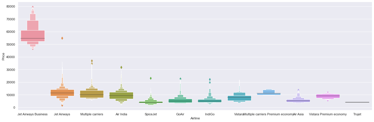
Only JetAirways Business having very high value, looks like an outlier
# Airline vs Price
sns.catplot(y = "Price", x = "Airline", data = train_data.sort_values("Price", ascending = False), kind="boxen", height = 6, aspect = 3)
plt.show()
# As Airline is Nominal data we will perform OneHotEncoding

Airline = train_data[["Airline"]]
Airline = pd.get_dummies(Airline, drop_first= True)
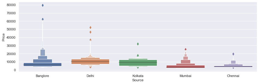
# Source vs Price

sns.catplot(y = "Price", x = "Source", data = train_data.sort_values("Price", ascending = False), kind="boxen", height = 4, aspect = 3)
plt.show()
Source = train_data[["Source"]]
Source = pd.get_dummies(Source, drop_first= True)
Destination = train_data[["Destination"]]
Destination = pd.get_dummies(Destination, drop_first = True)
Remove unwanted items as Route is related to stops and Additional info large margin is no_info
train_data.drop(["Route", "Additional_Info"], axis = 1, inplace = True)
Stops are Ordinal Values:
train_data.replace({"non-stop": 0, "1 stop": 1, "2 stops": 2, "3 stops": 3, "4 stops": 4}, inplace = True)
data_train = pd.concat([train_data, Airline, Source, Destination], axis = 1)
data_train.drop(["Airline", "Source", "Destination"], axis = 1, inplace = True)
Feature Selection:
Now we will try to do some basic feature selection process where we can identify the best usable features: Like correlation and feature importance etc. Will differentiate the features and labels, As it is a supervised machine learning problem.
y=data_train['Price']
X=data_train.drop(['Price'],axis=1)
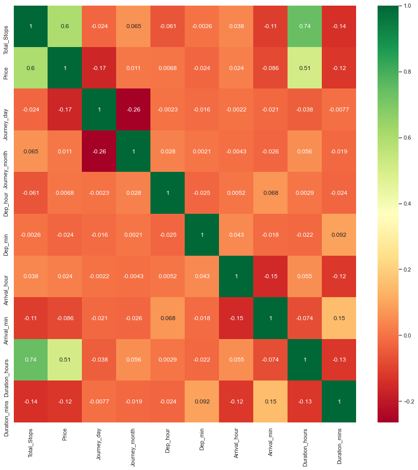
Heatmap to view correlated features:
plt.figure(figsize = (15,15))
sns.heatmap(train_data.corr(), annot = True, cmap = "RdYlGn")
plt.show()
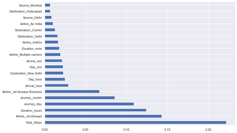
We will look important features using ExtraTreesRegressor
from sklearn.ensemble import ExtraTreesRegressor
selection = ExtraTreesRegressor()
selection.fit(X, y)
ExtraTreesRegressor()
Plot the graph for better visualization:
plt.figure(figsize = (12,8))
feat_importances = pd.Series(selection.feature_importances_, index=X.columns)
feat_importances.nlargest(20).plot(kind='barh')
plt.show()
Split the data into train and test:
from sklearn.model_selection import train_test_split
X_train, X_test, y_train, y_test = train_test_split(X, y, test_size = 0.2, random_state = 42)
Now time for the model selection: If we will do a multivariate analysis then we will get to know that the data is non-linear, and we have many categorical features. Decision Tree will work better in this scenario but it might be prone to overfit. Therefore we will go with RandomForestRegressor. We can also try with SVR also.
from sklearn.ensemble import RandomForestRegressor
reg_rf = RandomForestRegressor()
reg_rf.fit(X_train, y_train)
RandomForestRegressor()
y_pred = reg_rf.predict(X_test)
print(reg_rf.score(X_train, y_train))
print(reg_rf.score(X_test, y_test))
0.9516171822775591
0.790379004989978
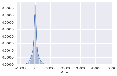
sns.distplot(y_test-y_pred)
plt.show()
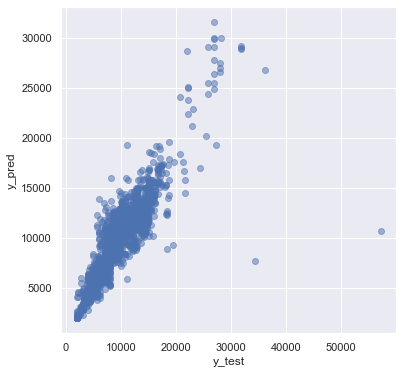
plt.scatter(y_test, y_pred, alpha = 0.5)
plt.xlabel("y_test")
plt.ylabel("y_pred")
plt.show()

Now we will look into the metrics figures:
from sklearn import metrics
print('MAE:', metrics.mean_absolute_error(y_test, y_pred))
print('MSE:', metrics.mean_squared_error(y_test, y_pred))
print('RMSE:', np.sqrt(metrics.mean_squared_error(y_test, y_pred)))
MAE: 1195.964437792086
MSE: 4519859.70113293
RMSE: 2125.9961667728685
Now we will do some hyperparameter tuning: Here we will use RondomizedSearchCV as it is comparitively fast.
from sklearn.model_selection import RandomizedSearchCV
# Number of trees in random forest
n_estimators = [int(x) for x in np.linspace(start = 100, stop = 1200, num = 12)]
# Number of features to consider at every split
max_features = ['auto', 'sqrt']
# Maximum number of levels in tree
max_depth = [int(x) for x in np.linspace(5, 30, num = 6)]
# Minimum number of samples required to split a node
min_samples_split = [2, 5, 10, 15, 100]
# Minimum number of samples required at each leaf node
min_samples_leaf = [1, 2, 5, 10]
# Random Grid
random_grid = {'n_estimators': n_estimators,
               'max_features': max_features,
               'max_depth': max_depth,
               'min_samples_split': min_samples_split,
               'min_samples_leaf': min_samples_leaf}
# Random search of parameters, using 5 fold cross validation,
# search across 100 different combinations
rf_random = RandomizedSearchCV(estimator = reg_rf, param_distributions = random_grid,scoring='neg_mean_squared_error', n_iter = 10, cv = 5, verbose=2, random_state=42, n_jobs = 1)
rf_random.fit(X_train,y_train)
Fitting 5 folds for each of 10 candidates, totalling 50 fits
[CV] n_estimators=900, min_samples_split=5, min_samples_leaf=5, max_features=sqrt, max_depth=10


[Parallel(n_jobs=1)]: Using backend SequentialBackend with 1 concurrent workers.


[CV]  n_estimators=900, min_samples_split=5, min_samples_leaf=5, max_features=sqrt, max_depth=10, total=   8.2s
[CV] n_estimators=900, min_samples_split=5, min_samples_leaf=5, max_features=sqrt, max_depth=10


[Parallel(n_jobs=1)]: Done   1 out of   1 | elapsed:    8.1s remaining:    0.0s


[CV]  n_estimators=900, min_samples_split=5, min_samples_leaf=5, max_features=sqrt, max_depth=10, total=   8.4s
[CV] n_estimators=900, min_samples_split=5, min_samples_leaf=5, max_features=sqrt, max_depth=10
[CV]  n_estimators=900, min_samples_split=5, min_samples_leaf=5, max_features=sqrt, max_depth=10, total=   8.3s
[CV] n_estimators=900, min_samples_split=5, min_samples_leaf=5, max_features=sqrt, max_depth=10
[CV]  n_estimators=900, min_samples_split=5, min_samples_leaf=5, max_features=sqrt, max_depth=10, total=   8.4s
[CV] n_estimators=900, min_samples_split=5, min_samples_leaf=5, max_features=sqrt, max_depth=10
[CV]  n_estimators=900, min_samples_split=5, min_samples_leaf=5, max_features=sqrt, max_depth=10, total=   8.3s
[CV] n_estimators=1100, min_samples_split=10, min_samples_leaf=2, max_features=sqrt, max_depth=15
[CV]  n_estimators=1100, min_samples_split=10, min_samples_leaf=2, max_features=sqrt, max_depth=15, total=  12.7s
[CV] n_estimators=1100, min_samples_split=10, min_samples_leaf=2, max_features=sqrt, max_depth=15
[CV]  n_estimators=1100, min_samples_split=10, min_samples_leaf=2, max_features=sqrt, max_depth=15, total=  12.5s
[CV] n_estimators=1100, min_samples_split=10, min_samples_leaf=2, max_features=sqrt, max_depth=15
[CV]  n_estimators=1100, min_samples_split=10, min_samples_leaf=2, max_features=sqrt, max_depth=15, total=  12.7s
[CV] n_estimators=1100, min_samples_split=10, min_samples_leaf=2, max_features=sqrt, max_depth=15
[CV]  n_estimators=1100, min_samples_split=10, min_samples_leaf=2, max_features=sqrt, max_depth=15, total=  12.7s
[CV] n_estimators=1100, min_samples_split=10, min_samples_leaf=2, max_features=sqrt, max_depth=15
[CV]  n_estimators=1100, min_samples_split=10, min_samples_leaf=2, max_features=sqrt, max_depth=15, total=  12.8s
[CV] n_estimators=300, min_samples_split=100, min_samples_leaf=5, max_features=auto, max_depth=15
[CV]  n_estimators=300, min_samples_split=100, min_samples_leaf=5, max_features=auto, max_depth=15, total=   8.0s
[CV] n_estimators=300, min_samples_split=100, min_samples_leaf=5, max_features=auto, max_depth=15
[CV]  n_estimators=300, min_samples_split=100, min_samples_leaf=5, max_features=auto, max_depth=15, total=   7.9s
[CV] n_estimators=300, min_samples_split=100, min_samples_leaf=5, max_features=auto, max_depth=15
[CV]  n_estimators=300, min_samples_split=100, min_samples_leaf=5, max_features=auto, max_depth=15, total=   7.9s
[CV] n_estimators=300, min_samples_split=100, min_samples_leaf=5, max_features=auto, max_depth=15
[CV]  n_estimators=300, min_samples_split=100, min_samples_leaf=5, max_features=auto, max_depth=15, total=   7.7s
[CV] n_estimators=300, min_samples_split=100, min_samples_leaf=5, max_features=auto, max_depth=15
[CV]  n_estimators=300, min_samples_split=100, min_samples_leaf=5, max_features=auto, max_depth=15, total=   8.1s
[CV] n_estimators=400, min_samples_split=5, min_samples_leaf=5, max_features=auto, max_depth=15
[CV]  n_estimators=400, min_samples_split=5, min_samples_leaf=5, max_features=auto, max_depth=15, total=  13.9s
[CV] n_estimators=400, min_samples_split=5, min_samples_leaf=5, max_features=auto, max_depth=15
[CV]  n_estimators=400, min_samples_split=5, min_samples_leaf=5, max_features=auto, max_depth=15, total=  13.7s
[CV] n_estimators=400, min_samples_split=5, min_samples_leaf=5, max_features=auto, max_depth=15
[CV]  n_estimators=400, min_samples_split=5, min_samples_leaf=5, max_features=auto, max_depth=15, total=  14.2s
[CV] n_estimators=400, min_samples_split=5, min_samples_leaf=5, max_features=auto, max_depth=15
[CV]  n_estimators=400, min_samples_split=5, min_samples_leaf=5, max_features=auto, max_depth=15, total=  14.2s
[CV] n_estimators=400, min_samples_split=5, min_samples_leaf=5, max_features=auto, max_depth=15
[CV]  n_estimators=400, min_samples_split=5, min_samples_leaf=5, max_features=auto, max_depth=15, total=  13.9s
[CV] n_estimators=700, min_samples_split=5, min_samples_leaf=10, max_features=auto, max_depth=20
[CV]  n_estimators=700, min_samples_split=5, min_samples_leaf=10, max_features=auto, max_depth=20, total=  22.0s
[CV] n_estimators=700, min_samples_split=5, min_samples_leaf=10, max_features=auto, max_depth=20
[CV]  n_estimators=700, min_samples_split=5, min_samples_leaf=10, max_features=auto, max_depth=20, total=  22.3s
[CV] n_estimators=700, min_samples_split=5, min_samples_leaf=10, max_features=auto, max_depth=20
[CV]  n_estimators=700, min_samples_split=5, min_samples_leaf=10, max_features=auto, max_depth=20, total=  22.0s
[CV] n_estimators=700, min_samples_split=5, min_samples_leaf=10, max_features=auto, max_depth=20
[CV]  n_estimators=700, min_samples_split=5, min_samples_leaf=10, max_features=auto, max_depth=20, total=  22.2s
[CV] n_estimators=700, min_samples_split=5, min_samples_leaf=10, max_features=auto, max_depth=20
[CV]  n_estimators=700, min_samples_split=5, min_samples_leaf=10, max_features=auto, max_depth=20, total=  22.6s
[CV] n_estimators=1000, min_samples_split=2, min_samples_leaf=1, max_features=sqrt, max_depth=25
[CV]  n_estimators=1000, min_samples_split=2, min_samples_leaf=1, max_features=sqrt, max_depth=25, total=  19.9s
[CV] n_estimators=1000, min_samples_split=2, min_samples_leaf=1, max_features=sqrt, max_depth=25
[CV]  n_estimators=1000, min_samples_split=2, min_samples_leaf=1, max_features=sqrt, max_depth=25, total=  19.7s
[CV] n_estimators=1000, min_samples_split=2, min_samples_leaf=1, max_features=sqrt, max_depth=25
[CV]  n_estimators=1000, min_samples_split=2, min_samples_leaf=1, max_features=sqrt, max_depth=25, total=  20.1s
[CV] n_estimators=1000, min_samples_split=2, min_samples_leaf=1, max_features=sqrt, max_depth=25
[CV]  n_estimators=1000, min_samples_split=2, min_samples_leaf=1, max_features=sqrt, max_depth=25, total=  20.1s
[CV] n_estimators=1000, min_samples_split=2, min_samples_leaf=1, max_features=sqrt, max_depth=25
[CV]  n_estimators=1000, min_samples_split=2, min_samples_leaf=1, max_features=sqrt, max_depth=25, total=  19.9s
[CV] n_estimators=1100, min_samples_split=15, min_samples_leaf=10, max_features=sqrt, max_depth=5
[CV]  n_estimators=1100, min_samples_split=15, min_samples_leaf=10, max_features=sqrt, max_depth=5, total=   6.8s
[CV] n_estimators=1100, min_samples_split=15, min_samples_leaf=10, max_features=sqrt, max_depth=5
[CV]  n_estimators=1100, min_samples_split=15, min_samples_leaf=10, max_features=sqrt, max_depth=5, total=   6.7s
[CV] n_estimators=1100, min_samples_split=15, min_samples_leaf=10, max_features=sqrt, max_depth=5
[CV]  n_estimators=1100, min_samples_split=15, min_samples_leaf=10, max_features=sqrt, max_depth=5, total=   6.7s
[CV] n_estimators=1100, min_samples_split=15, min_samples_leaf=10, max_features=sqrt, max_depth=5
[CV]  n_estimators=1100, min_samples_split=15, min_samples_leaf=10, max_features=sqrt, max_depth=5, total=   6.7s
[CV] n_estimators=1100, min_samples_split=15, min_samples_leaf=10, max_features=sqrt, max_depth=5
[CV]  n_estimators=1100, min_samples_split=15, min_samples_leaf=10, max_features=sqrt, max_depth=5, total=   6.8s
[CV] n_estimators=300, min_samples_split=15, min_samples_leaf=1, max_features=sqrt, max_depth=15
[CV]  n_estimators=300, min_samples_split=15, min_samples_leaf=1, max_features=sqrt, max_depth=15, total=   3.3s
[CV] n_estimators=300, min_samples_split=15, min_samples_leaf=1, max_features=sqrt, max_depth=15
[CV]  n_estimators=300, min_samples_split=15, min_samples_leaf=1, max_features=sqrt, max_depth=15, total=   3.1s
[CV] n_estimators=300, min_samples_split=15, min_samples_leaf=1, max_features=sqrt, max_depth=15
[CV]  n_estimators=300, min_samples_split=15, min_samples_leaf=1, max_features=sqrt, max_depth=15, total=   3.3s
[CV] n_estimators=300, min_samples_split=15, min_samples_leaf=1, max_features=sqrt, max_depth=15
[CV]  n_estimators=300, min_samples_split=15, min_samples_leaf=1, max_features=sqrt, max_depth=15, total=   3.2s
[CV] n_estimators=300, min_samples_split=15, min_samples_leaf=1, max_features=sqrt, max_depth=15
[CV]  n_estimators=300, min_samples_split=15, min_samples_leaf=1, max_features=sqrt, max_depth=15, total=   3.3s
[CV] n_estimators=700, min_samples_split=10, min_samples_leaf=2, max_features=sqrt, max_depth=5
[CV]  n_estimators=700, min_samples_split=10, min_samples_leaf=2, max_features=sqrt, max_depth=5, total=   4.3s
[CV] n_estimators=700, min_samples_split=10, min_samples_leaf=2, max_features=sqrt, max_depth=5
[CV]  n_estimators=700, min_samples_split=10, min_samples_leaf=2, max_features=sqrt, max_depth=5, total=   2.9s
[CV] n_estimators=700, min_samples_split=10, min_samples_leaf=2, max_features=sqrt, max_depth=5
[CV]  n_estimators=700, min_samples_split=10, min_samples_leaf=2, max_features=sqrt, max_depth=5, total=   3.5s
[CV] n_estimators=700, min_samples_split=10, min_samples_leaf=2, max_features=sqrt, max_depth=5
[CV]  n_estimators=700, min_samples_split=10, min_samples_leaf=2, max_features=sqrt, max_depth=5, total=   4.3s
[CV] n_estimators=700, min_samples_split=10, min_samples_leaf=2, max_features=sqrt, max_depth=5
[CV]  n_estimators=700, min_samples_split=10, min_samples_leaf=2, max_features=sqrt, max_depth=5, total=   4.3s
[CV] n_estimators=700, min_samples_split=15, min_samples_leaf=1, max_features=auto, max_depth=20
[CV]  n_estimators=700, min_samples_split=15, min_samples_leaf=1, max_features=auto, max_depth=20, total=  26.0s
[CV] n_estimators=700, min_samples_split=15, min_samples_leaf=1, max_features=auto, max_depth=20
[CV]  n_estimators=700, min_samples_split=15, min_samples_leaf=1, max_features=auto, max_depth=20, total=  26.0s
[CV] n_estimators=700, min_samples_split=15, min_samples_leaf=1, max_features=auto, max_depth=20
[CV]  n_estimators=700, min_samples_split=15, min_samples_leaf=1, max_features=auto, max_depth=20, total=  25.6s
[CV] n_estimators=700, min_samples_split=15, min_samples_leaf=1, max_features=auto, max_depth=20
[CV]  n_estimators=700, min_samples_split=15, min_samples_leaf=1, max_features=auto, max_depth=20, total=  25.7s
[CV] n_estimators=700, min_samples_split=15, min_samples_leaf=1, max_features=auto, max_depth=20
[CV]  n_estimators=700, min_samples_split=15, min_samples_leaf=1, max_features=auto, max_depth=20, total=  25.6s


[Parallel(n_jobs=1)]: Done  50 out of  50 | elapsed: 10.4min finished


RandomizedSearchCV(cv=5, estimator=RandomForestRegressor(), n_jobs=1,
                   param_distributions={'max_depth': [5, 10, 15, 20, 25, 30],
                                        'max_features': ['auto', 'sqrt'],
                                        'min_samples_leaf': [1, 2, 5, 10],
                                        'min_samples_split': [2, 5, 10, 15,
                                                              100],
                                        'n_estimators': [100, 200, 300, 400,
                                                         500, 600, 700, 800,
                                                         900, 1000, 1100,
                                                         1200]},
                   random_state=42, scoring='neg_mean_squared_error',
                   verbose=2)
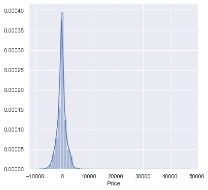
prediction = rf_random.predict(X_test)
plt.figure(figsize = (6,6))
sns.distplot(y_test-prediction)
plt.show()
plt.figure(figsize = (6,6))
plt.scatter(y_test, prediction, alpha = 0.5)
plt.xlabel("y_test")
plt.ylabel("y_pred")
plt.show()
print('MAE:', metrics.mean_absolute_error(y_test, prediction))
print('MSE:', metrics.mean_squared_error(y_test, prediction))
print('RMSE:', np.sqrt(metrics.mean_squared_error(y_test, prediction)))
MAE: 1165.9884093683927
MSE: 4129107.8069248367
RMSE: 2032.020621678047
Save Model:
Now finally we will save the model, as we know that model is an object so we will use the concept of serialization to persistant storage through the python pickle and reuse it whenever required.
import pickle
# open a file, where you ant to store the data
file = open('flight_rf.pkl', 'wb')
# dump information to that file
pickle.dump(reg_rf, file)

# Deserialize and use the model object
model = open('flight_rf.pkl','rb')
forest = pickle.load(model)
y_prediction = forest.predict(X_test)
metrics.r2_score(y_test, y_prediction)
0.790379004989978
This is a very basic implementation of a regression model. We can also improve our accuracy in many ways like by investigating more into the EDA part and try with different regression algorithms and fine tune them.